3. Pandas
Python is filled with functions to do pretty much anything you’d ever want to do with a programming language: navigate the web, parse data, interact with a database, run fancy statistics, build a pretty website and so much more.
Creative people have put these tools to work to get a wide range of things done in the academy, the laboratory and even in outer space. Some are included in a toolbox that comes with the language, known as the standard library. Others have been built by members of Python’s developer community and need to be downloaded and installed from the web.

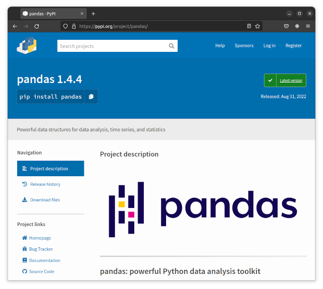
One third-party tool that’s important for this class is called pandas. It was invented for use at a financial investment firm and has become the leading open-source library for accessing and analyzing data in many different fields.
3.1. Import pandas
Create a new cell at the top of your notebook where we will import pandas for our use. Type in the following and hit the play button.
Show code cell content
my_list = [1, 3, 5, 7, 9, 999]
import pandas
If nothing happens, that’s good. It means you have pandas installed and ready to use.
Note
Since pandas is created by a third party independent from the core Python developers, it wouldn’t be installed by default if you followed our advanced installation instructions.
It’s available to you because the JupyterLab Desktop developers have pre-selected a curated list of common utilities to include with the package, another reason to love their easy installer.
If your notebook doesn’t have pandas, you can install it by running %pip install pandas in a cell. This will download and install the library using the pip package manager and Jupyter’s built-in magic command.
Return to the cell with the import and rewrite it like this.
import pandas as pd
This will import the pandas library at the shorter variable name of pd. This is standard practice in the pandas community. You will frequently see examples of pandas code online using pd as shorthand. It’s not required, but it’s good to get in the habit so that your code is more likely to be quickly understood by other computer programmers.
Note
In Python, a variable is a way to store a value in memory for later use. A variable is a named location in the computer’s memory where a value can be stored and retrieved. Variables are used to store data values, such as numbers, strings, lists, or objects, and they can be used throughout the program to refer to the stored value.
To create your own variable in Python, you use the assignment operator (=) to assign a value to a variable. The variable name is on the left side of the assignment operator and the value is on the right side.
3.2. Conduct a simple data analysis
Those two little letters contain dozens of data analysis tools that we’ll use in future lessons. They can read in millions of records, compute advanced statistics, filter, sort, rank and do just about anything else you’d want to do with data.
As we saw with the list in the last chapter, Python can do quite a bit on its own. The advantage of pandas is that it saves time by offering even more options.
We can start to get a look at its powers by converting that plain Python list into what pandas calls a Series. Here’s how to make it happen in your next cell. Let’s stick with simple variables and name it my_series.
my_series = pd.Series(my_list)
Once the data becomes a Series, you can immediately run a wide range of descriptive statistics. Let’s try a few.
How about summing all the numbers? Make a new cell and run this. It should spit out the total, just like the sum() function in the last chapter.
my_series.sum()
np.int64(1024)
Then find the maximum value in the next.
my_series.max()
np.int64(999)
The minimum value in the next.
my_series.min()
np.int64(1)
How about the average?
my_series.mean()
np.float64(170.66666666666666)
And how about the median, which we didn’t have a way to do with just Python?
my_series.median()
np.float64(6.0)
Let’s go further. How about the standard deviation?
my_series.std()
np.float64(405.8086577029458)
Finally, all of the above, plus a little more about the distribution, in one simple command.
my_series.describe()
count      6.000000
mean     170.666667
std      405.808658
min        1.000000
25%        3.500000
50%        6.000000
75%        8.500000
max      999.000000
dtype: float64
If you substituted in a series of 10 million records, your notebook would calculate all those same statistics without you needing to write any more code. Once your data, however large or complex, is imported into pandas, there’s little limit to what you can do to filter, merge, group, aggregate, compute or chart using simple methods like the ones above. In the chapter to come we’ll start doing just using that with data from a real Los Angeles Times investigation.